Data Compression with Arithmetic Coding

Lossless and lossy data compression methods both employ the arithmetic coding process often. The approach uses entropy encoding, where symbols that are seen more frequently require fewer bits to encode than symbols that are seen less frequently. Compared to popular approaches like Huffman coding, it offers several benefits. You will have a thorough knowledge of all the specifics required to perform arithmetic coding from this article’s detailed description of the CACM87 implementation.

Introduction

Lossless data compression employs a type of entropy encoding known as arithmetic coding (AC). As with the ASCII code, a string of characters is often represented using a set number of bits per character. The number of bits utilized overall will decrease when a string is converted to arithmetic encoding because frequently occurring characters will be stored with fewer bits and less often occurring characters will be stored with more bits.

Arithmetic coding is distinct from other types of entropy encoding, like Huffman coding, in that it only encodes the entire message into a single number, an arbitrary-precision fraction q, where 0.0 q 1.0, as opposed to breaking the input up into individual symbols and replacing each with a code. A range that is specified by two integers serves as a representation of the most recent data. Because they work directly on a single natural number that represents the most recent information, the asymmetric numeral systems family of entropy coders, which is relatively new, enables quicker implementations.

Lossy techniques for data compression reduce data while sacrificing certain information. Even while this lowers the quality of the reconstructed data, it lessens the number of bits utilized to represent the message.

Without any loss, lossless algorithms recreate the original data. In comparison to lossy algorithms, they employ more bits as a result.
A lossless approach called arithmetic encoding (AE) employs a few bits to compress data.
It is an entropy-based approach that was initially put out in a 1987 work by Ian H. Witten, Radford M. Neal, and John G. Cleary titled “Arithmetic coding for data compression” Communications of the ACM 30.6 (1987): 520–540.

The fact that AE techniques only use one integer between 0.0 and 1.0 to encode the whole message contributes to the reduction in bits. According to its likelihood, each symbol in the message is assigned a sub-interval in the range of 0 to 1.

A frequency table should be provided to the algorithm as input in order to compute the likelihood of each symbol. Each character is mapped to its frequency in this table.

The symbol’s allotted bits decrease as its frequency increases. As a result, there is a decrease in the overall number of bits needed to represent the complete message. In Huffman coding, all of the symbols in the message are represented by a set number of bits.

Encoding with Floating Point Math

In computing, floating-point arithmetic (FP) is arithmetic that approximates real values using formulaic representation in order to provide a trade-off between range and precision. Due to the need for quick processing speeds, systems with extremely tiny and very large real numbers frequently employ floating-point calculation. A floating-point number is often approximated by having a given number of significant digits (the significand), and it is scaled using an exponent in a fixed base, which is typically two, ten, or sixteen.

The phrase “floating point” describes a number’s ability to “float,” or to be positioned wherever in relation to the significant digits of the number. A number’s radix point, also known as the decimal point or, more frequently in computers, the binary point, can be used to represent a number. The floating-point format may be viewed as a type of scientific notation because the exponent serves as a marker for this place.

The diameter of an atomic nucleus or the distance between galaxies may both be stated using the same unit of length in a floating-point system, which can represent quantities of multiple orders of magnitude with a fixed number of digits.

It is necessary to utilize Scientific or Floating-point notation for encoding non-integer numbers. Although there are several floating-point systems, the IEEE 754 standard is one of the more popular ones.
A mantissa and an exponent are the two main parts of a value represented in floating-point format. For the IEEE 754 standard, the actual structure of these is investigated.

There are several ways to handle floating-point values: entirely in software, using a separate “math co-processor” chip, or using intricate instructions integrated into the main processor. Floating-point is an integral part of the CPU in the majority of contemporary desktop and laptop computers. Although the software-emulated floating point is much, much slower than the hardware-emulated floating point, it may be programmed to maintain higher accuracy or range than the underlying hardware.

Examining the Floating Point Prototype

In the project that is attached, fp proto.CPP, the first pass encoder is illustrated. I also needed to define a basic model in order to get it running. I’ve developed a model in this instance that can encode 100 letters, each with a fixed probability of .01 and beginning with the letter “A” in the first place. I’ve just developed the class enough to encode the capital letters from the ASCII character set in order to keep things simple:

struct {
  static std::pair<double,double> getProbability( char c )
  {
    if (c >= 'A' && c <= 'Z')
      return std::make_pair( (c - 'A') * .01, (c - 'A') * .01 + .01);
    else
      throw "character out of range";
  }
} model;

As a result, in this probability model, “A” owns the range from 0.0 to 0.01, “B” owns the range from .01 to .02, “C” owns the range from .02 to .03, and so on. I invoked this encoder with the string “WXYZ” as an illustrative example. Let’s go over what occurs in the encoder step by step.

High and low are initially set to 1.0 and 0.0, respectively. When the encoder requests the probabilities for the letter “W,” the model responds with the interval [0.22, 0.23], which represents the portion of the probability line that “W” controls in this model. You can see that low is now set to 0.22 and high is set to 0.23 by moving your cursor over the following two lines.

If you look at how this works, you’ll find that high will always be bigger than low despite the fact that the gap between high and low gets narrower as each letter is decoded. In addition, the value of low is continually rising while the value of high is always falling. For the algorithm to operate properly, several invariants are crucial.

The final number in the message will thus be less than .23 and higher than or equal to .22 once the first character has been encoded, regardless of the remaining values that are encoded. Both the low and the high will be strictly less than the other, with the low being bigger than the high and less than the low but less than the high. This means that no matter what occurs after this, we will be able to identify the initial character during decoding since the final encoded number will fall inside the range held by ‘W,’ according to this rule. The figure below illustrates the narrowing process roughly:

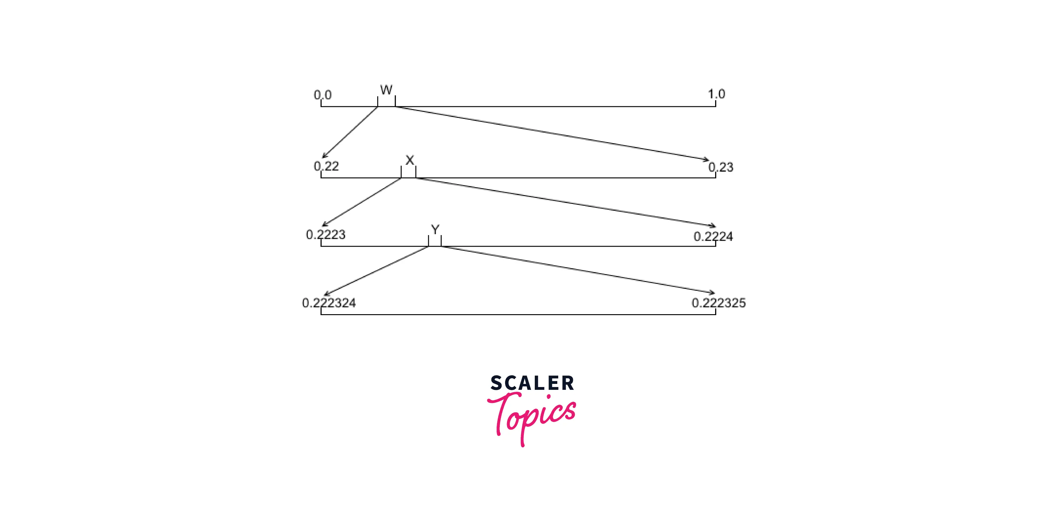
Let’s examine the second character, the letter “X,” to observe how this limiting functions. For this character, the model yields a range of [.23,.24], and the high and low values are then recalculated to provide an interval of [.2223,.2224]. Thus, the high and low are still inside the original[.22,23] range, but the gap has shrunk.

The output appears as follows after the inclusion of the final two characters:

Encoded message: 0.2223242550

Theoretically, for this specific message, any floating point number in the range [0.22232425,0.2223242] should correctly decode to the necessary values. I’ll go into more detail about how the precise value we want to output has to be picked.

Decoding with Floating Point Math

The encoding algorithm is quite simple in my opinion. The decoder reverses the procedure; it is not more difficult, but the stages might not be as evident. A first-pass decoding method for this message might be like the following:

void decode(double message)
{
  double high = 1.0;
  double low = 0.0;
  for ( ; ; ) 
  {
    double range = high - low;
    char c = model.getSymbol((message - low)/range);
    std::cout << c;
    if ( c == 'Z' )
      return;
    std::pair<double,double> p = model.getProbability(c);
    high = low + range * p.second;
    low = low + range * p.first; 
  }
}

In essence, the arithmetic from the encode side is reversed in the decoder. The probability model just has to locate the character whose range includes the current value of the message to decode a character. The model detects that the sample value of 0.22232425 fits inside the [0.22,0.23] interval owned by ‘W,’ the model outputs W when the decoder initially starts up. The decoder part of the basic model is represented as follows in fp proto.CPP:

static char getSymbol( double d)
{
  if ( d >= 0.0 && d < 0.26)
    return 'A' + static_cast<int>(d*100);
  else
    throw "message out of range";
}

As each character is processed in the encoder, the output value range is continuously narrowed. The segment of the message we are looking at in the decoder to find the next character is similarly constrained. High and low now constitute an interval of [0.22,0.23], with a range of .01, after the decoding of the “W.” Because of this, the method used to determine the next probability value to be decoded, (message – low)/range, will result in a value of.2324255, which falls exactly in the middle of the range covered by “X”.

As the letters are decoded, this narrowing keeps going until the letter “Z,” which is the hardcoded end of the message, is reached. Success!

Unbounded Precision Math with Integers

You will have to get your head around some unusual maths in this, the second section of the presentation. Although variables of type double will no longer be used to accomplish the method that was explained in the first section of this article, it will still be accurately carried out. Instead, integer variables and math will be used to implement it, although in creative ways.

The fundamental idea that we put into practice is that high, low, and the actual encoded message will all have values that are binary integers with an infinite length. As a result, both high and low as well as the output value itself will be millions of bits long by the time Moby Dick has been fully encoded for Project Gutenberg. Each of the three will continue to signify a number less than one, larger than zero, and equal to three.

An even more intriguing aspect of this is that despite the fact that each of the three values in question is millions of bits long, processing a character just requires a small number of operations using 32 bits, or maybe 64 bits if you like, of simple integer math.

Number Representation

Remember how low and high were started in the reference implementation of the algorithm:

 double high = 1.0;
 double low = 0.0;

We change to a representation like this for the algorithm’s integer variant:

 unsigned int high = 0xFFFFFFFFU;
 unsigned int low = 0;

Since there is an inferred decimal point before both numbers, it follows that high is really (0.FFFFFFFF in hex, or 0.1111…111 in binary), while low is 0.0. The inferred decimal point before the first bit in the number that we produce will be the same.

This, however, is not exactly accurate because the high in the initial implementation was 1.0. In terms of proximity to 1.0, the value is 0.FFFFFFF is only a little below. What will be done about this?

In this case, certain mathematically challenging concepts are used. High contains 32 memory bits, yet we still think of it as having an indefinitely long trail of binary 1s trailing off the right end. Therefore, it is not merely 0. They are there but haven’t yet been moved into memory, as seen by the series of Fs (or 1s) that goes on forever, ending in FFFFFFFF.

Although it may not be immediately apparent, Google may assist in persuading you that a limitless series of 1s beginning with 0.1 is actually equivalent to 1. (The quick version is: x = 1.0 since x = 2x – x.) Low is likewise thought of as an endlessly long binary string with 0s dangling off the end to the very last binary position.

Resulting Changes to the Model

Integer math will be used exclusively in the final implementation, so keep that in mind. Prior to now, the model had the ability to deliver probabilities as a pair of floating point integers that represented the range that a certain symbol owned.

A symbol still owns a particular range of numbers on the number line that is higher than or equal to 0 and less than 1 in the modified version of the method. However, we’ll now use the fractions upper/denim and lower/denom to illustrate this. Our model code is not much impacted by this. For the letter “W,” for instance, the sample model from the preceding section returned .22 and .23. Instead, it will now return a structure named prob with the values 22, 23, and 100.

A Sample Implementation

The production code included in ari.zip combines all of this information. LINK. This code is quite versatile because of the usage of templates, which should make it simple to integrate into your own applications. The header files provide all the necessary code, making project inclusion straightforward.

I’ll go over the many elements that must come together in order to do compression in this part. Four programs are included in the code package:

• The floating point prototype program is called fp proto.CPP. useful for testing new ideas but not for doing actual work.
• Using command line options, compress.cpp compresses a file.
• Using command line options, a file is decompressed using the program decompress.cpp.
• Using tester.cpp, a file is placed through a compress/decompress cycle, the validity is checked, and the compression ratio is displayed.

All of the template classes in header files that make up the compression code are used to implement it. These are:

• The arithmetic compressor is fully implemented in the compressor.h. Model type, input stream type, and output stream type are all parameters for the compressor class.
• The comparable arithmetic decompressor with the same type argument is decompressor.h.
• modelA.h, a straightforward order-0 model that successfully illustrates compression.
• A model class can set up some types utilized by the compressor and decompressor with the aid of the utility class model metrics.h.
• The streaming classes that implement bit-oriented I/O are bitio.h and byteio.h.

The information is relevant to the bit-oriented I/O classes implemented in bitio.h and byteio.h will not be covered in detail in this article. The classes are easy to adapt for different kinds and allow you to read or write from std::iostream and FILE * sources and destinations. In my essay C++ Generic Programming Meets OOP, which uses a bit-oriented I/O class as an example, I go into further detail on how these classes are implemented.

Conclusion

• The first aspect of arithmetic coding to comprehend is the results. A message (typically a file) made up of symbols is converted into a floating point number larger than or equal to zero and less than one using arithmetic coding. These symbols are almost usually eight-bit characters. This floating point number is not a typical data type that you are used to utilizing in traditional programming languages since it may be rather large—in fact, your whole output file is one long number.
• The second aspect of arithmetic coding to comprehend is that in order to characterize the symbols it is processing, it uses a model. The model’s role is to inform the encoder of the likelihood of each character in a given message. They will be encoded almost exactly ideally if the model predicts the message’s characters with a high degree of accuracy. Your encoder could enlarge a message instead of compressing it if the model misrepresents the probability of symbols!
• It uses an entropy encoding approach in which more bits are used to encode often-seen symbols than seldom-seen symbols.
• An explanation of how arithmetic coding works using common C++ data types to construct floating point arithmetic. This enables a totally reasonable, if perhaps impractical, approach. In other words, it functions, but it is limited to relatively brief message encoding.
• The advantage of lossless compression is that the input sequence may be precisely recreated from the encoded sequence. A lossless encoding may be created using the statistical coding method known as arithmetic coding, which is almost ideal.
• An arithmetic encoder will unquestionably have more computing needs than a method like Huffman, but the effect this has on your software should be as little as possible thanks to contemporary CPU architectures. Comparing Huffman coding with arithmetic encoding, we find that the former is particularly suitable for adaptive models.
• For the safe transfer of data, encoding is the process of transforming the data—or a specific sequence of letters, symbols, alphabets, etc.—into a predetermined format.