The right view of binary tree is the set of nodes seen by an observer as standing to the right of a given binary tree. The nodes visible to the observer will be the rightmost nodes at each level. All the other nodes (which will lie to the left of the rightmost nodes) will be hidden since they will lie behind the rightmost nodes in their respective levels.
Scope of Article
This article discusses
- Problem statement for the right view of the binary tree
- Approaches to print the right view of a given binary tree in data structures:
- Recursive (or Depth-first Search) approach
- Iterative (or Breadth-first search) approach
- Program implementation of the above-mentioned approaches in
C++andPython - Complexity analysis of the algorithms used
Takeaways
Time and Space complexity:
- Time Complexity:
O(n) - Space Complexity :
O(n)
Introduction
Imagine you’re a Star Wars character leading a bunch of Resistance spaceships to attack a First Order base called the Death Tree (similar to the Death Star).
You command your troopers to get in a linear formation and attack the base at once. The launched missiles hit the base on the right side at once as shown.
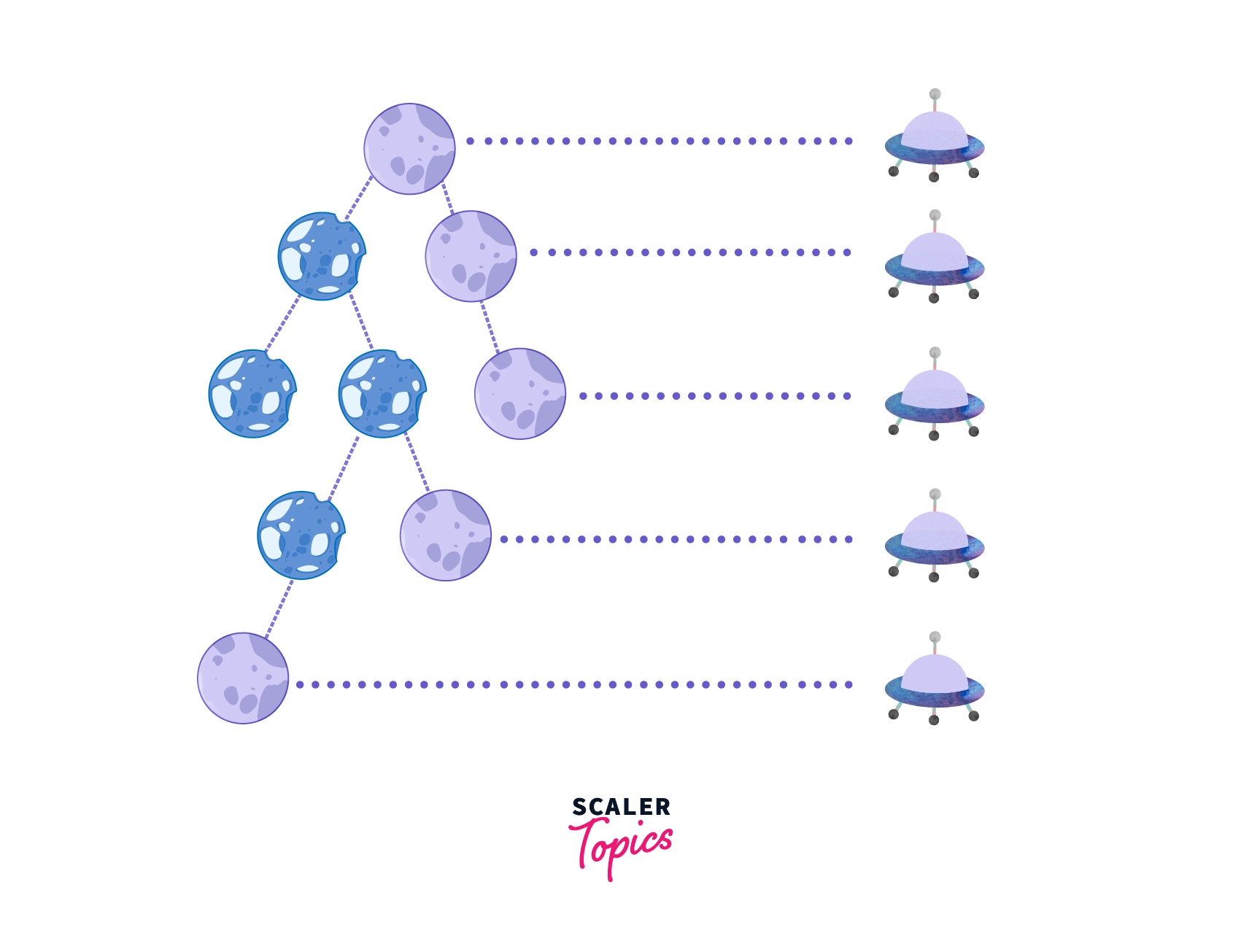
The set of nodes where the explosion is taking place makes up the right view of binary tree. Having gained a visual introduction, let us describe the right view of the binary tree in the upcoming section.
What is the Right View of Binary Tree?
The right view of binary tree is the part of the tree observed by an observer standing right to the tree and facing it.
Therefore, the right view consists of the rightmost nodes of each valid level of the tree.
But, what is a level?
We can define the level of a binary tree as the set of nodes that have an equal number of edges between themselves and the root node (that is, nodes equidistant from the root).
For example, consider the tree with root node as 1:
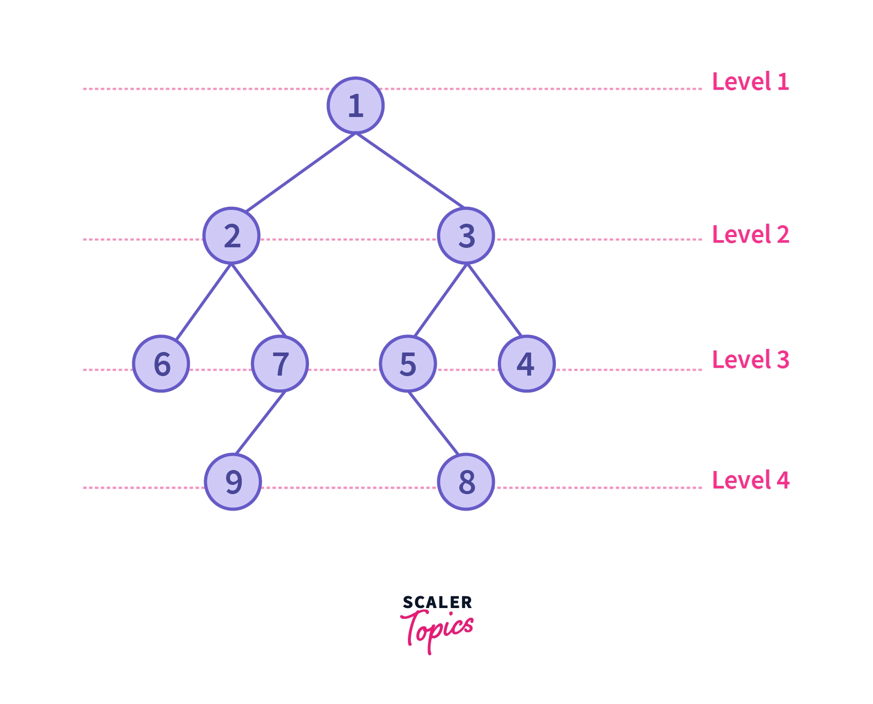
The nodes present in each level are given as:
| Level | Nodes |
|---|---|
| 0 | 1 |
| 1 | 2, 3 |
| 2 | 6, 7, 5, 4 |
| 3 | 9, 8 |
Please note that you can start labelling the levels from either 0 or 1.
Example of Right View of Binary Tree
Consider again the tree we used above. As we said earlier, the rightmost node of each level will be part of our right view of the binary tree. That is:
| Level | Nodes | Rightmost Node |
|---|---|---|
| 0 | 1 | 1 |
| 1 | 2, 3 | 3 |
| 2 | 6, 7, 5, 4 | 4 |
| 3 | 9, 8 | 8 |
Therefore, the right view of the binary tree is
1 3 4 8Or, visually, the right view of the binary tree is as follows:
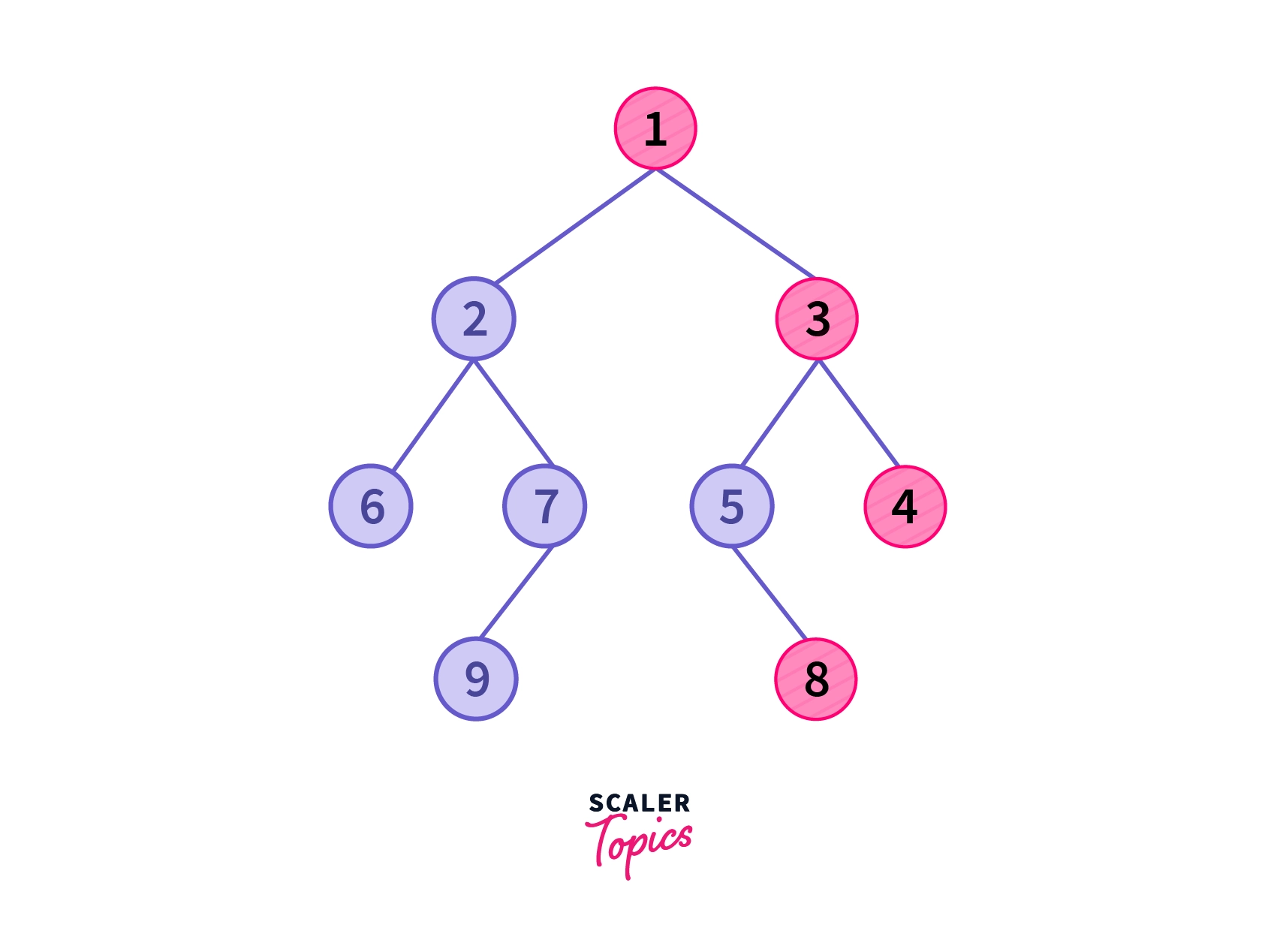
Taking another example, consider the tree shown below:
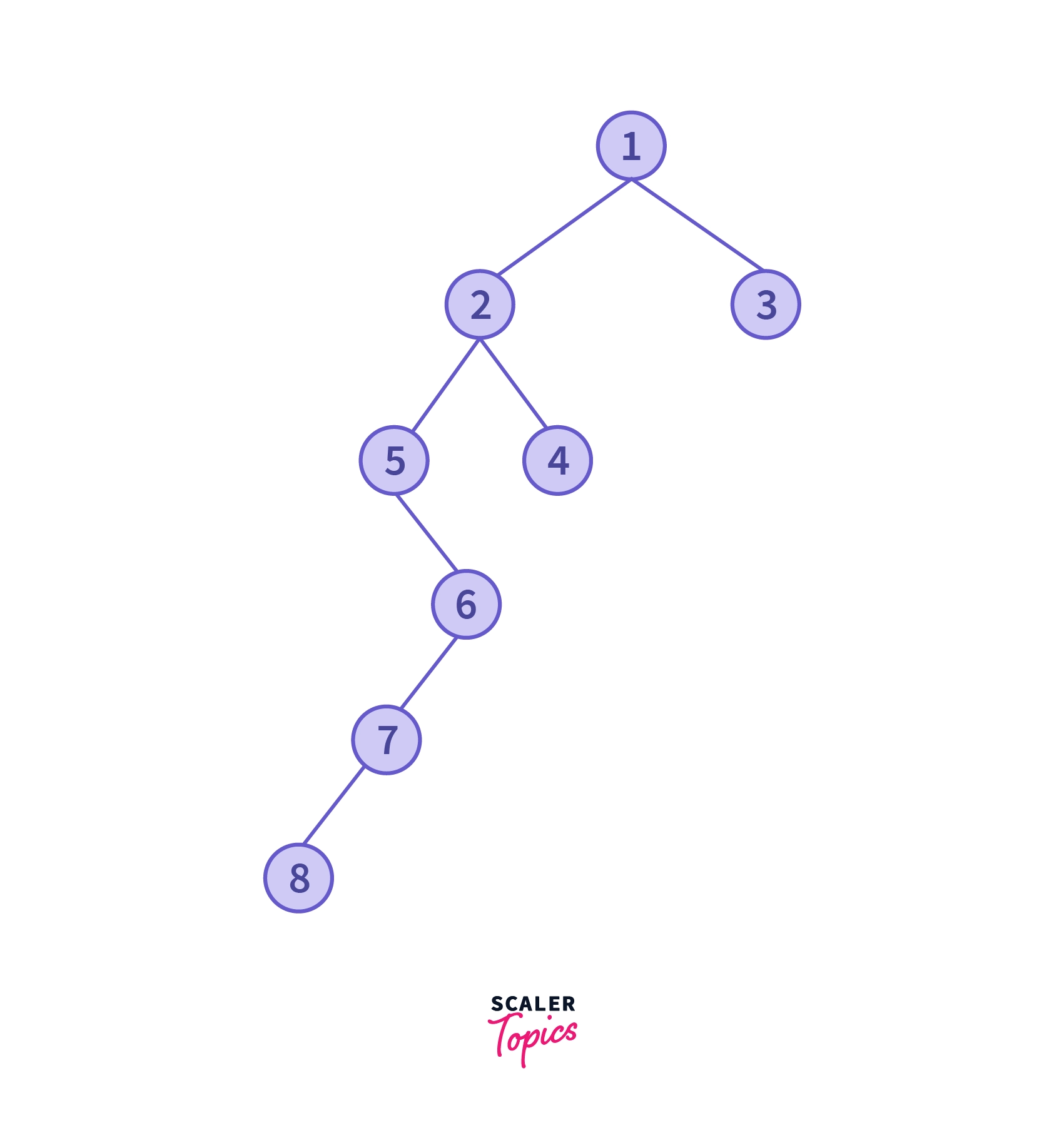
| Level | Nodes | Rightmost Node |
|---|---|---|
| 0 | 1 | 1 |
| 1 | 2, 3 | 3 |
| 2 | 5, 4 | 4 |
| 3 | 6 | 6 |
| 4 | 7 | 7 |
| 5 | 8 | 8 |
Therefore, the right view of the given binary tree is
1 3 4 6 7 8Algorithm
There are two approaches to solve this problem, one is recursive (depth-first-search based) approach, while the other is iterative (breadth-first-search based) approach.
Recursive / DFS Approach
Intuition
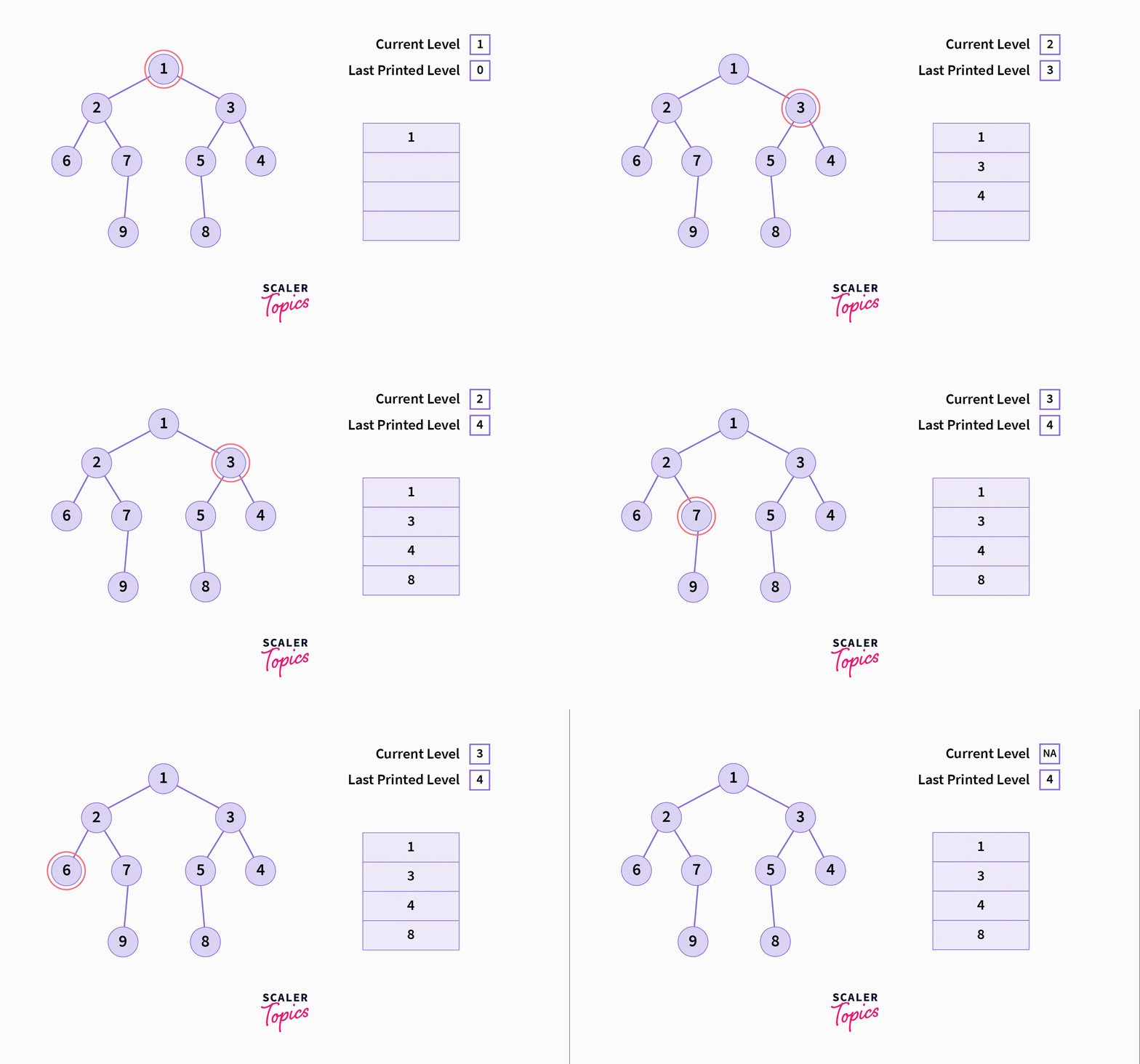
DFSis one of the most basic traversal techniques for a graph/tree, therefore, we can try solving our problem using it.- Suppose I am in a given level, it appears that the algorithm should consider the right subtree with higher importance than the left one, since we have to print the rightmost node. This can be achieved by a right-oriented pre-order traversal, that is, current node, followed by right subtree, followed by the left subtree.
- In any given level, the algorithm must ONLY print the rightmost node, and if it has been printed, the algorithm must not print any other node (in that level).
- It can be achieved by using a variable which keeps track of the last level for which the rightmost node has been printed.
- Now, if that variable’s value is less than the value of the given level, it means that we are in a level whose rightmost node has not been printed. Therefore, we must print whatever node we first encounter/process in this level.
- Since our traversal is right oriented (see point 2), then we will always reach the rightmost node of a level before other nodes of that level.
Now, let’s see the algorithm where we used all the points we discussed above.
The Recursive Algorithm
- Initialize two variables: a.
curr_level: The current level of the tree we are currently present in during the traversal b.last_printed_level: The last level for which the rightmost node has been printed/stored. - Process the following sequentially in a recursive manner: a. Current node b. Right subtree c. Left subtree
- At the current node (if it is not null) check whether the
current level > last printed level. a. If Yes: Print / store the current node and update the value oflast_printed_leveltocurr_level. b. If No: Continue - Before calling the function recursively on the right and left subtree, increase the value of
levelby1.
Note:
The variable last_printed_level should either be a global variable (not recommended) or be passed by reference to function calls (recommended). This is done to ensure that the current level is compared to most recently updated value of last_printed_level.
Please see the animated gif below to for a better visual understanding of the algorithm.
Iterative / BFS Approach
Intuition
This, perhaps, is the most intuitive way of solving this problem.
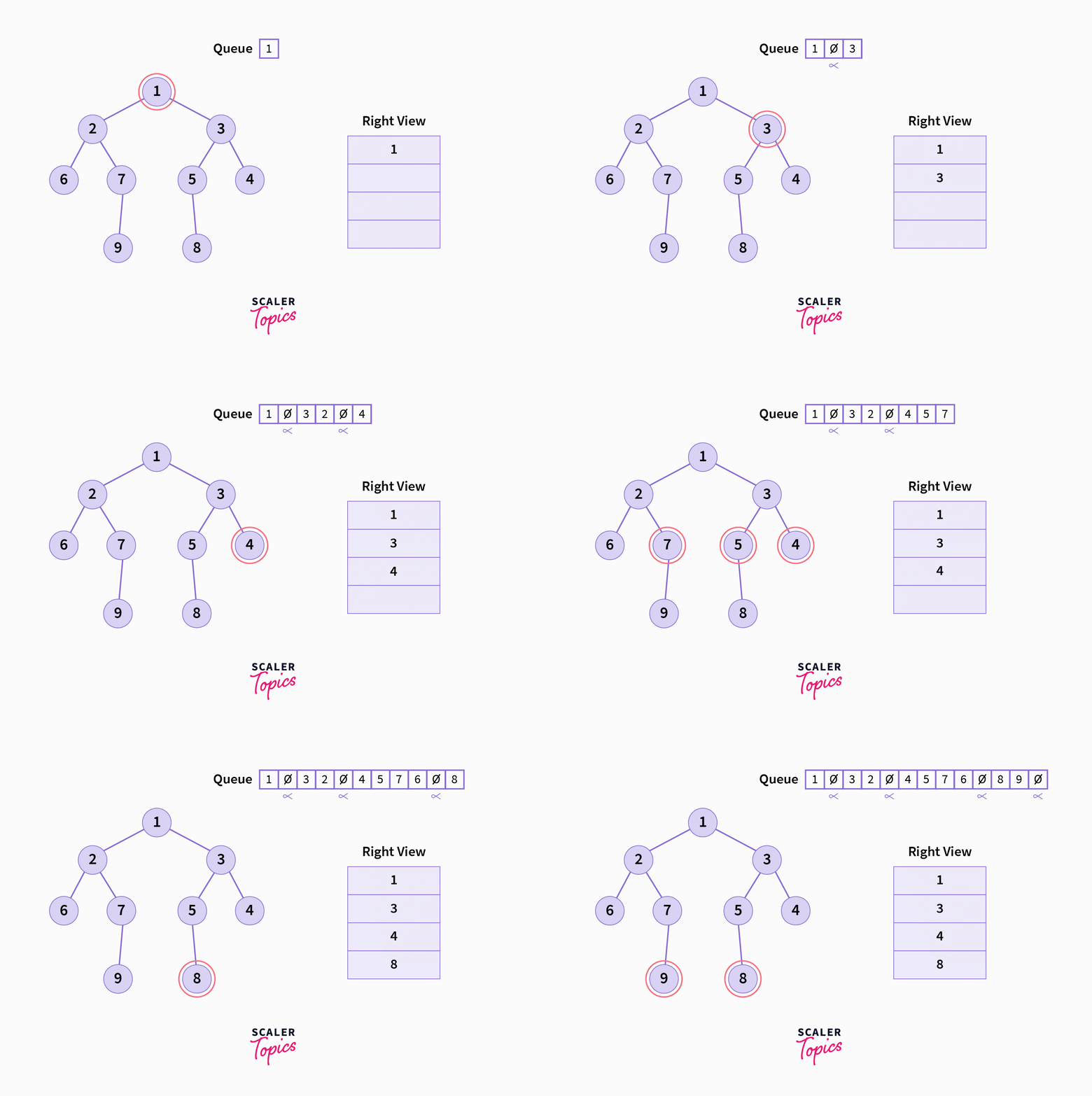
- We travel the entire tree level by level (from right to left).
- At each level, we print/store the right most node.
- After the algorithm is done processing the entire tree, we will obtain the right view of the binary tree given to us.
The Iterative Algorithm
- Initialize a queue data structure ((commonly used in BFS algorithm) with the root node and a
LevelEndcharacter to mark a level’s end in the queue. Commonly,nullptrorNULLis used asLevelEndin C/C++, whileNoneis used in Python. - While the queue is not empty, do the following: a. Pop the front of the queue, and call it
frontValb. IffrontValisLevelEnd, and the resultant queue is not empty, pop and print the front value of the resultant queue (this is the rightmost node of the given level), and also push aLevelEndcharacter into the queue. c. IffrontValisLevelEndand the resultant queue is empty, break out of the while loop. d. IffrontValis notLevelEnd, then push its right child followed by left child into the queue (they must exist, of course).
Explanation
- The above stated algorithm is just a right-oriented version of the standard
Level-Order-Traversalalgorithm. - Between any two
LevelEndcharacters, an entire level of the given tree is present (except, of course, thelevel 0, that is, the root node) - Since we give priority to the right child node over the left child node while pushing into the queue (see step 2.c of the algorithm) we ensure that the queue contains levels in a right to left fashion with respect to the binary tree given.
- Because of the above point, we can be sure that the node just after the
LevelEndcharacter in the queue is the rightmost node in the given binary tree’s level. Therefore, we printed it in step (2.b) of the algorithm.
Note:
Please note that it is not necessary to push the right child first. If we had pushed the left child of the current node into the queue, then in step (2.b) we would print the node just before the LevelEnd characters instead of other way round.
The reason for this is that the resultant queue will contain levels in left to right fashion with respect to the given binary tree.
See the animated gif given below for a better visual understanding of the algorithm.
Right View Of Binary Tree: Code Implementation
Before you see the code solution below, it is recommended that you try to implement the above-discussed algorithms yourself here on InterviewBit.
C++ (DFS Approach)
/*
Definition for a binary tree node.
struct TreeNode
{
    int val;
    TreeNode *left;
    TreeNode *right;
};
*/


// utility function
void right_view_util(TreeNode* root, int &last_printed_level, int curr_level)
{
    // if root is null, there is nothing to do
    if(root==nullptr)
    {
        return;
    }

    if(last_printed_level<curr_level)
    {
        cout << root->val <<" ";
        last_printed_level = curr_level;
    }

    right_view_util(root->right, last_printed_level, curr_level+1);
    right_view_util(root->left, last_printed_level, curr_level+1);

    return;
}

void print_right_view(TreeNode* root)
{
    int curr_level = 1;
    int last_printed_level = 0;

    // print the right view
    right_view_util(root, last_printed_level, curr_level);

    return;
}
Explanation
- As explained in the algorithm, the code traverses the given tree in the fashion (
current node-> right subtree->left subtree). - At each node, if the
last_printed_level<curr_level, we print the current level. - To keep the value of the variable
last_printed_levelup-to-date, we pass it by reference to each recursive call.
Python (DFS Approach)
# Definition for the node of a binary tree
# class TreeNode:
#     def __init__(self, val=0, left=None, right=None):
#         self.val = val
#         self.left = left
#         self.right = right

def right_view_util(root, last_printed_level, curr_level):

    if(root==None):
        return

    # if current level has not been printed
    if(last_printed_level[0]<curr_level):
        print(root.val)
        last_printed_level[0] = curr_level

    right_view_util(root.right, last_printed_level, curr_level+1)
    right_view_util(root.left, last_printed_level, curr_level+1)

    return

def print_right_view(root):

    curr_level = 1
    last_printed_level = [0]

    # print the right view
    right_view_util(root, last_printed_level, curr_level)

    return
C++ (BFS Approach)
/*
Definition for a binary tree node.
struct TreeNode
{
    int val;
    TreeNode *left;
    TreeNode *right;
};
*/

void print_right_view(TreeNode* root)
{
    if(root==nullptr)
    {
        return;
    }

    // declaring an empty queue for Level Order Traversal
    queue<TreeNode*> Q;

    // the first level of the tree
    Q.push(root);
    Q.push(nullptr);

    // printing the root
    cout << root->val << " ";

    // processing the rest of the tree
    while(!Q.empty())
    {
        TreeNode* front = Q.front();

        // if front is nullptr
        // it means that current level has ended
        if(front==nullptr)
        {
            Q.pop();
            if(!Q.empty())
            {
                // print the value of the front node
                cout << Q.front()->val <<" ";
                Q.push(nullptr);
            }

            continue;
        }


        // since this node is not the rightmost node
        // remove it from the queue
        Q.pop();


        // add the next nodes to the queue
        // with right node having higher priority
        if(front->right!=nullptr)
        {
            Q.push(front->right);
        }
        if(front->left!=nullptr)
        {
            Q.push(front->left);
        }

    }

    return;
}
Explanation
- A queue is initialized which can store node pointer values.
- We perform a right-oriented level-order traversal. Therefore, after popping out a
LevelEndcharacter, the next value in queue is the rightmost node of the level we are currently processing in the queue. So, we print it and pop it from the queue. - Rest all the nodes are not printed.
Python (BFS Approach)
# Definition for the node of a binary tree
# class TreeNode:
#     def __init__(self, val=0, left=None, right=None):
#         self.val = val
#         self.left = left
#         self.right = right

def print_right_view(root):
        if not root:
            return

        # declaring a queue
        node_queue = collections.deque()
        node_queue.append(root)
        node_queue.append(None)

        # print the root
        print(root.val, end = ' ')

        # process the rest of the tree
        while node_queue:
            front_node=node_queue.popleft()

            if front_node==None:
                if not node_queue:
                    break
                else:
                    print(node_queue[0].val, end=' ')
                    node_queue.append(None)
                    continue

            if front_node.right:
                node_queue.append(front_node.right)

            if front_node.left:
                node_queue.append(front_node.left)
Complexity Analysis
- Time Complexity: Since all the nodes are processed exactly once, therefore if the number of nodes present in the tree is of order $n$, then the time complexity of both the algorithms we used to find the right view of the binary tree is:
$$
\mathcal{O}(n)
$$
- Space Complexity:
a.DFS Solution: $\mathcal{O}(h)$, where $h$ is the height of the binary tree
b.BFS Solution: $\mathcal{O}(n)$, where $n$ is the order of number of nodes in the binary tree
Conclusion
Right viewofbinary treeconsists of the rightmost nodes of each level in the binary tree.- Two methods can be used to obtain the right view of binary tree; one uses a
DFSapproach, and the other uses aBFSapproach. - While using the
DFS(recursive) approach, we keep track of the level we are currently in, and the last level for which we have already obtained the rightmost node. - While using the
BFS(iterative) approach, we perform a level order traversal and store/print the rightmost node in any given level.