Sorting Algorithms

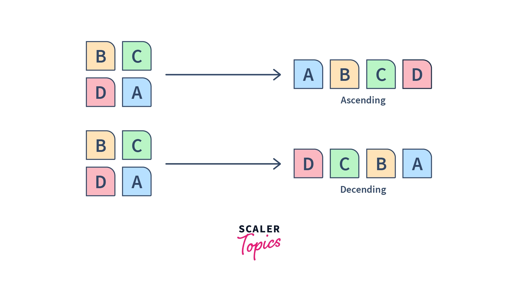
Sorting refers to the process of arranging a list or a sequence of given elements(that can be numbers or strings, etc.) or data into any particular order, which may be ascending or descending.
Sorting is basically useful whenever we want our data to be in an ordered form. To make our lives easier, we have sorting algorithms to perform the given tasks of sorting our data. The Sorting algorithms are a defined set of rules or processes by which we can easily sort our list or array. In this article, we are going to learn about what is sorting.

Scope

This article deals with “what is sorting”. Throughout the article, we are going to cover the following points in brief:

• How different sorting algorithms work and how they compare under different situations
• Importance of sorting algorithms
• Time and space complexity of sorting algorithms
• In-place and Not-in-place Sorting
• Stable and Not Stable Sorting
• Adaptive and Non-Adaptive Sorting Algorithm
• Sorting Categories like Internal & External Sorting
• The Efficiency of the sorting algorithms
• Time and space complexity trade-off in sorting algorithms

By the end of this article, you will understand sorting algorithms from both a theoretical and a practical standpoint. We are also going to cover the code snippets for them.

Overview of Sorting

Suppose, you are trying to find the phone number of your friend in a call-book diary of 100 pages, containing around 500 contact number details. Now, if all of the contacts are arranged in a haphazard manner, without any particular order, then it might take you the whole day to find out the contact detail of 1 person.

So, this is where sorting comes into the picture. If the contact names would be arranged in a manner where their names were alphabetically sorted, then it might have taken less than a min to find out the contact number.

So, sorting is the process using which we arrange our data in a particular order, be it ascending or descending. There are ample sorting algorithms that help us in doing this task.

Example

Since sorting is often capable of reducing the algorithmic complexity of some particular types of problems, it has found its usage in a wide range of fields. Some of them are discussed below.

• Dictionary: The dictionary stores words in alphabetical order so that searching for any word becomes easy.
• Telephone Book: The telephone book stores the telephone numbers of people sorted by their names in alphabetical order, so that the names can be searched easily.
• E-commerce application: While shopping through any e-commerce application like amazon or flipkart, etc. , we preferably tend to sort our items based on their price range, popularity, size, etc.

Also, the sorting algorithm’s real-life usage is just miraculous! For example —

• Quick sort is used for updating the real-time scores of various sports.
• Bubble sort is used in TV to sort the channels based on audience viewing timings.
• Merge Sort is very popularly used by databases to load a huge amount of data.

Sorting Algorithms

A sorting algorithm is an algorithm that puts elements of a list into order. The most frequently used orders are numerical order, where the elements are arranged on the basis of their numerical value. Another order of sorting is the lexicographical order, where elements are arranged alphabetically. In simple words, Lexicographical order is nothing but the dictionary order or preferably the order in which words appear in the dictionary.

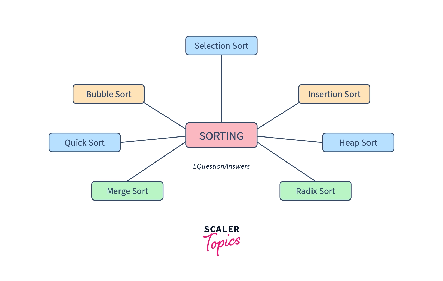
There are various sorting algorithms, which we will learn in our next article.

Importance of Sorting Algorithms

Sorting algorithms are the backbone of many programming solutions. They are widely used in computer science due to the following reasons:

• Reduce the computational complexity of various problems.
• Make raw data simpler and meaningful to analyze. Because, after sorting any list or array, we get our data in an ordered form. Hence it becomes simpler to analyze them.
• Make it easier to implement search algorithms to find or retrieve an item from a dataset efficiently and perform operations on them.
• Sorting helps us to solve most of the problems which require an ordered set of data. For example, it is easier for us to check our score(or marks) from any list, because the list is sorted either lexicographically(based on our names), or numerically(based on our roll numbers).

Time and Space complexity

Time Complexity

Time complexity in the programming world measures the approximate time taken by a piece of code, or algorithm to execute(or run) based on the size of input passed to it.

Time complexity does not give us the exact measure of time, but it gives us an overall estimation of the time taken.

The time taken mainly depends upon the number of times lines of code will iterate.

Time complexity Notations:
These are the asymptotic notations that are used for calculating the time complexity of the sorting algorithms:

1. Big oh Notation, O: It measures the upper limit of an algorithm’s running time or the worst-case time complexity. It is known by $O(n)$ for input size ‘n’.
2. Omega Notation, Ω: It measures the minimum time taken by algorithms to execute, and calculates the best case time complexity in sorting. It is known by $Ω(n)$ for input size ‘n’.
3. Theta Notation, θ: It measures the average time taken by an algorithm to execute. Or, the lower bound and upper bound of an algorithm’s running time. It is known by $θ(n)$ for input size ‘n’.

Few examples on worst-case time complexity may include:

• $O(1)$ means constant time complexity. It means, that no matter what the size of the input is, the time taken to compute it will always be constant. Below code takes constant time.

#calculates the sum of first
#n natural numbers
def sumOfNumbers(n):
    #directly implement the formula
    s = (n*(n+1))//2
    return s

#driver code
print(sumOfNumbers(10))  #55 

• $O(N)$ means linear time complexity, for an input of size N. For example the below code takes linear time because the loop iterates over the length ‘n’ only once.

fact = 1
n = 5
for i in range(1,n+1):
    fact = fact * i
print(fact) #55

• The time complexity of $O(log N)$ algorithm is logarithmic time complexity. The below code has a logarithmic time complexity.

Code:

n = 1024
while n > 0:
    print(n, end = '')
    # every time the value of n 
    # gets halved
    n //= 2

# Output:
# 1024 512 256 128 64 32 16 8 4 2 1

• If our code has a big-Oh time complexity of $O(N^2)$ or $O(N^3)$, etc. then that means it has quadratic time complexity.

Space Complexity:

Space Complexity is the total memory space required by any program for the execution of its code. It depends on the size of the data structure we are using to do our code. The sorting algorithms which take constant space are also known as the in-place sorting algorithms. If we do not use any data structure(eg. array, list etc.) then our code uses constant space. $O(1)$ specifies constant space complexity. Other parameters like linear, quadratic, or exponential space complexity are similar like what we defined for our time complexity.

In-place Sorting and Out-of-place Sorting

In-place Sorting:

• An In-place algorithm modifies the inputs, which can be a list or an array, without using any additional memory. As the algorithm runs, the input is usually overwritten by the output, so no additional space is required.
• However, the in-place sorting algorithms may take some memory, like using some variables, etc. for its operation. Overall, it takes constant memory for its operation.
• Sorting algorithms such as insertion sort, selection sort, quick sort, bubble sort, heap sort, etc. use in-place sorting. They don’t require any extra space and rearrange the input in the same array.
• Since they take constant space, the space complexity of these algorithms is $O(1)$.

Out-of-place Sorting:

• An algorithm that is not in place is called a not-in-place or out-of-place algorithm. The Out-of-place sorting algorithm uses extra space for sorting, which depends upon the size of the input.
• The standard merge sort algorithm is an example of the out-of-place algorithm as it requires O(n) extra space for merging.

Stable and Not Stable Sorting

Suppose we are sorting any list or array, and we have some duplicate elements in it, at some given positions(or indexes). If we use any stable sorting algorithm to sort the data, then the relative positions(or order) of the duplicate elements will not be altered.

Let us say, we have two $5’s$ in a given array, one at the $2^{\text{nd}} index$ and another at $7^{\text{th}} index$. After sorting, the $5$ at $index = 2$ will always remain before the $5$ at $index = 7$ , irrespective of their position after sorting. This is possible if we use a stable sorting algorithm to sort the array.

More formally, the stability of a sorting algorithm is related to how the algorithm treats equal (or repeated) elements. Whether it maintains their relative order(the order in which they are present in the input) while sorting or not. Based on this, we have 2 types of algorithms:

1. Stable Sorting:

• The Stable sorting algorithms preserve the relative order of equal elements. In other words, they maintain the relative position of similar elements after sorting.
• If we have a key-value pair in our list, then in the case of stable sort original order of equal keys is maintained.
• Several common sorting algorithms are stable by nature, such as Merge Sort, Timsort, Counting Sort, Insertion Sort, and Bubble Sort. We will read about them further in this tutorial.
• Stability is important when we have key-value pairs with duplicate or equal keys. It is however not so important when all the elements are different.
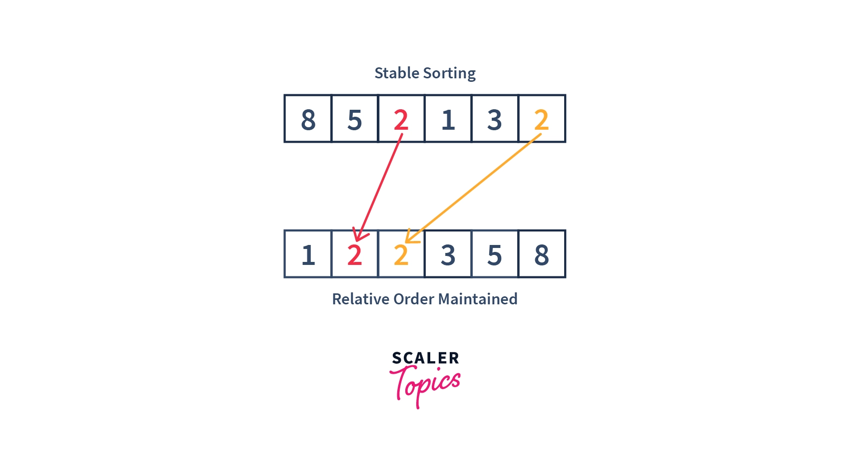
• Below image shows how stable sorting works:

In the above image, we have two $2’s$ at different positions in our array. One at the $2^{\text{nd}} index$ and another at $5^{\text{th}} index$ (considering indexing starts from $0^{\text{th}} index$). After sorting them, the resultant $2’s$ are at $1^{\text{st}} index$ and $2^{\text{nd}} index$ respectively.

But please note, the $2$ which was at the $2^{\text{nd}} index$ initially (before sorting) remains before the $2$ which was at $5^{\text{th}} index$ initially. Hence, we may say that the relative order of the elements were preserved after sorting, using a stable sorting algorithm.

2. Non-Stable Sorting:

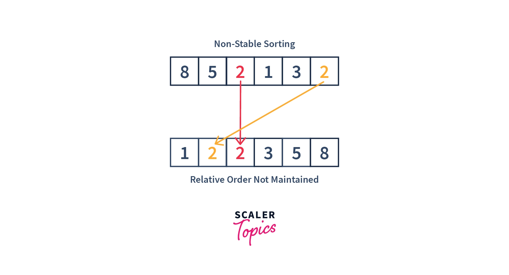
• In a Non-Stable sorting algorithm the ordering of the same values is not necessarily preserved/maintained after sorting.
• Whenever there are no duplicates in our data set, then non-stable or stable sorting elements do not make any difference. This is because the stability of the sorting algorithm is dependent upon the factor that whether the relative positions of the same elements are maintained or not after sorting. So, if there are no duplicate elements at all, then, there is no need of comparing the relative positions themselves.
• Selection sort, Shell sort, Quicksort, and Heapsort may be considered an example of Non-Stable sorting algorithms.
• Below image shows how non-stable sorting works:

Adaptive and Non-Adaptive Sorting Algorithm

In certain sorting algorithms, the complexity of sorting changes with the order of input given (pre-sorted or completely unsorted). Based on this, we have the following categories:

Adaptive Sorting:

• If the order of the elements to be sorted of an input array matters (or) affects the time complexity of a sorting algorithm, then that algorithm is called the “Adaptive” sorting algorithm.
• Since the order of the input affects the adaptive sorting algorithms, adaptive sort takes advantage of the existing order of the input to try to achieve better computational time complexity. In other words, the more presorted the input is, the faster it should be sorted.
• For example – Quick sort is an adaptive sorting algorithm because its time complexity depends on the initial input’s sequence or order. If the input is already sorted then time complexity becomes $O(n^2)$ and if the input sequence is not given in a sorted form then time complexity becomes $O(n logn)$.
• Examples of Adaptive Sorting algorithms may include Bubble Sort, Insertion Sort and Quick Sort.

Non-Adaptive Sorting:

• In Non-Adaptive Sorting, the order of the elements in the input array does not matter, the time complexity remains always the same for any order of the given input.
• Some non-adaptive sorting algorithms are: Selection Sort, Merge Sort, and Heap Sort.

The Efficiency of Sorting Algorithms

• Sorting algorithms are judged in terms of their efficiency. Time complexity and space complexity are a few of the other factors(we have discussed below) that largely impact the efficiency of any algorithm.
• Efficiency refers to the “algorithmic efficiency” as the size of the input grows large. The algorithmic efficiency is generally based on the number of elements to sort.
• Algorithms should be judged based on their average case, best case, and worst case efficiency (which we discussed above). Because many algorithms that have the same efficiency do not have the same speed on the same input.
• Some algorithms, such as quicksort, perform exceptionally well for some inputs but are highly time taking for other inputs. Certain algorithms, such as merge sort, are unaffected by the order of input data. So, the efficiency of certain algorithms differs as per the input given to them, while for some algorithms it doesn’t matter.
• One more important factor is the constant term $C$, which we generally ignore while calculating the time complexities, for example, $O(C*n)$ is just $O(n)$. But the constant, $C$, will vary across different algorithms. For example, the constant factor for a quick sort algorithm is far smaller than that of the heapsort.
• Space requirement is another important feature to measure the efficiency of algorithms. As we discussed above, factors such as are they in-place or out-of-place algorithms and the data structure used for them also determine their space requirement. The in-place algorithms use constant memory, whereas the out-of-place algorithms use memory based on the data structure, etc. used. Hence, they deeply affect the space requirement of any algorithm.
• Finally, the stability(whether the order of the elements is preserved while sorting) of the algorithms also determines their efficiency, which we discussed above in detail.

Sorting Categories

Sorting is again divided into two categories – Internal and External sorting, let’s discuss below:

Internal Sorting:

• If the data sorting process takes place entirely within the RAM of a computer, it is called internal sorting.
• Internal sorting is only possible whenever the size of the list or the data to be sorted is small enough to be stored in the RAM of our machine. We can only perform internal sorting when our size of data is small enough to be fitted in our main memory.
• For example, bubble sort will work best if we store the whole chunk of our data in the main memory at once. If we do not do this, then continuously moving data in and out of memory will lead to performance degradation. Hence, internal sorting is preferred here.
• Some algorithms which use internal sorting may include bubble sort, insertion sort, quick sort, etc.

External Sorting:

• Eternal sorting is used, whenever we need to sort very large datasets, which may not be stored in the memory as a whole at once.
• So, for sorting larger datasets, we may hold only a smaller chunk of data in memory at a time, since it won’t all fit in the RAM at once.
• And, the rest of the data is normally stored in some other(slower) memory like the hard disk.
• External sort usually requires algorithms whose space complexity doesn’t increase with the size of the dataset.

In short, we use internal sorting when the dataset is relatively small enough to fit within the RAM of the computer. For example, bubble sort, Insertion sort and quick sort can be sorted internally. And external sorting is used when the dataset is large and hence uses algorithms that have minimum space complexity. An example of external sorting is the external merge sort algorithm, which is a K-way merge algorithm. It sorts chunks that each fit in RAM and then merges the sorted chunks together.

Other Characteristics of Sorting algorithms

We have already discussed all the important characteristics and classifications of sorting algorithms. However, there are a few other characteristics of sorting algorithms that cannot be missed. Let’s discuss them:

1. Comparison Sort: Comparison sorting algorithms are those which work by comparing each pair of adjacent elements of an iterable(such as list, array, etc.) using any comparison operator(suppose > or < or =). Some sorting algorithms are comparison sort while others are not.

For example, heap sort is a comparison sort, whereas counting sort isn’t. Bubble sort, Insertion sort, Merge sort, heap sort etc. are comparison-based sorting algorithms. Whereas, count sort, radix sort, and bucket sort are not comparison-based.

2. Parallelism: Sorting algorithms are either serial or parallel. A parallel algorithm can do multiple operations at a time, whereas the serial sorting algorithms work on one operation at a time. The serial sorting algorithms work like, one operation is executed only after the previous operation is completed. We can consider the example of merge sort where two sequences say $X$ and $Y$ can only be merged once they are sorted. This is a kind of serial algorithm implementation. An example of a parallel algorithm is, that we can easily implement bucket sort to sort buckets in parallel. Bucket sort is a parallel sorting algorithm because we can sort the buckets parallelly.
3. Recursive: Some algorithms are recursive by nature, for example, the merge sort or quick sort, use the divide and conquer technique to solve the problem. This makes them more of a recursive sorting algorithm. It allows for the sorting of $n$ elements in $O(N log N)$ time compared with the $O(n^2)$ efficiency of bubble sort. Hence, recursive techniques can be utilized in sorting algorithms.

Trade-Offs of Sorting Algorithms

The space and time complexity of an algorithm are the major determinants of its efficiency. To make the algorithm more efficient, we consistently try to reduce both the time and space complexity. 

But unfortunately, this is not always possible because of the underlying trade-off between the time and space complexity of any sorting algorithm. By that, we mean that, whenever we are trying to reduce one of them (time or space), the other factor(such as time or space) usually increases. Suppose, if we are trying to optimize the space, then the time complexity might increase and vice versa. Hence, we may say there is a trade-off between the sorting algorithms where we can prioritize one of the time and space complexity and implement our algorithm.

Conclusion

In this article, we got an in-depth idea about sorting algorithms. Let’s just recap what we learned throughout:

• Sorting means arranging our data into a particular order. We have ample sorting algorithms to perform this.
• Time complexity of the sorting algorithms determines the overall estimated time that will be taken to run an algorithm of size ‘n’.
• In place sorting is when the sorting algorithm does not use any extra memory for sorting, whereas out-of-place sorting algorithms use extra memory.
• Stable sorting algorithms maintain the relative order of their inputs whereas unstable sorting algorithms do not.
• Adaptive algorithms depend upon the initial arrangement of the dataset given(already sorted or not), whereas non-adaptive algorithms do not.
• Internal sorting takes place when we sort data in our RAM itself, whereas in external sorting, the data consumes extra memory to be sorted.
• Efficiency of a sorting algorithm depends upon various factors such as time complexity, space complexity, the constant factor, stability, adaptivity, and the size of the input.
• There is a trade-off between time and space complexity in sorting algorithms.